Simulations

goal: simulate fault-free PRAMs on fault-prone PRAMs
preserve the efficiency of the original algorithm
processors are subject to fail-stop failures
Following two cases have equal complexity:
- execution of a single \(N\)-processor PRAM step on \(P\) fail stop processors
- solving \(N\)-size write-all problem using \(P\) fail-stop processors

Fault tolerant PRAM

(definition)

given arbitrary failure pattern \(f\) of failure model \(F\)
fault-free PRAM \(A\)
PRAM \(B\) that tolerates failures of \(F\)

PRAM is fault-tolerant when any sequence of instructions of \(A\) can be executed on \(B\) in the precense of any failure pattern \(f \in F\).

Simulation efficiencies

Simulation is

optimal for \(F\) if \(S = O(N \cdot \tau)\)
robust for \(F\) if \(S = O(N \cdot \tau \cdot \log^cN)\) for constant \(c\)
polynomial for \(F\) if \(S = O(N \cdot \tau \cdot N^\epsilon)\) for a constant \(\epsilon\), \(0 < \epsilon < 1\)

Example: GPA simulation

This simple example uses general parallel assignment (GPA) problem:
- inputs:
  1. array \(y[1...N]\)
  2. function \(f\)
- in parallel, compute for each value in y: \(y[PID] = f(\text{PID}, y[1...N])\)
- assume cost of \(f\) is \(O(1)\)

Failure-free solution

shared int array y[1...N]; // each initialized to Y_i
forall PID = 1...N parbegin
  y[PID] = f(PID, y[1...N])
parend
// function f has been applied to elements of y

Fault-tolerant version

Assume surviving processors can be reassigned to unfinished tasks.

1. convert assignment to idempotent form

solution must accommodate multiple attempts to write by different processors at different times. Assignments are made idempotent by introducing two generations of array \(y\) and using binary generation version numbers:

shared int array y[0...1][1...N];
private bit integer v (init 0)
forall PID = 1...N parbegin
  y[v+1][PID] = f(PID, y[v][1...N])
  v = v + 1 (mod 2)
parend
// f has been applied to elements of y[v]

values of the first generation array are used as input
computed values are stored in the second generation array
the binary version number is incremented after all assignments

2. Modify robust write-all algorithm

Assume \(R\) is a robust algorithm for write-all. Make following changes to \(R\):

before each x[e] = 1 for some variable e, insert: y[v+1][e] = f(e, y[v][1...N])
insert statement to increment v before HALT statement of each processor's code

to obtain \(R'\).

correctness of \(R'\) follows from correctness of \(R\)
assignments to \(y\) do not affect write-all computation
when \(R\) terminates, so does \(R'\)

=> complexity of solving GPA is equal to complexity of solving write-all.

Implications:

use any write-all and appropriate function \(f\) to perform any single parallel computation step in presence of failures by copying \(N\) computed values from one array to another
to simulate arbitrary parallel step: use iterative parameterized approach:
- targets of assignment correspond to memory locations written by simulated processors
- \(f\) represents machine instructions executed by the simulated processors

PRAM interpreter

Goal: construct fault-tolerant PRAM interpreter
This same methodology can be used to
- simulate parallel algorithms or
- transform parallel algorithms to robust algorithms
interpreter can execute any standard PRAM models (CRCW, CREW... etc.)
if we are able to simulate PRAM interpreter in another parallel/distributed model, then any PRAM program also becomes program in that model.
If we understand: 1. efficiency of PRAM program and 2. complexity of simulating PRAM interpreter in another model → able to evaluate efficiency of the program in the context of another model

Pseudo code of the PRAM interpreter (failure free)

forall processors PID=1..P parbegin
    shared SM[1..m];            // shared memory
    shared PROG[1..P ,1..size]; // P programs of length size
    private IB                  // instruction buffer

  private r record              // private registers
    IC                          // instruction counter
    RR                          // read register (a buffer)
    WR                          // write register (an address)
    ... end                     // up to polylog of general-purpose registers
  r.IC := 1;                    // start at the first instruction

  while r.IC != 0 do            // while not HALT
    IB                          // fetch into IB
    r.RR                        // read cycle
    r                           // compute
    SM[W (r)]                   // write
    r.IC                        // next instruction
  od
parend

PRAM interpreter definition

has \(P\) processors
processors have unique PIDs from 1 to \(P\)
each processor has:
- instruction buffer (IB)
- internal registers \(r\) (number of registers per \(P\), \(|r|\) is \(l\))
- \(r\) contains:
  - instruction counter (IC)
  - a read register (RR)
  - write register (WR)
shared array PROG[1..P,1..size] stores instructions of a compiled PRAM program (size does not depend on P)
- program per processor is PROG[i,1..size] with on instruction per array element
uses shared memory cells \(SM[1 \dots m]\)
- first \(N\) cells contain input for the compiled program
- cells and registers can store \(O(\log max\{N,P\})\) bits each
Instruction set \(\{R, C, W, J\}\), and instruction cycle:
1. read instruction into IB
2. read into RR contents of \(SM[R(r)]\)
3. assign to r result og computation C(r)
4. write contents of WR to shared memory \(SM[R(r)]\)
5. update instruction counter; if IC=0 then HALT.

Regarding memory,

The instructions are stored in memory and address of next instruction in IC.
private memory is typically larger than in a uniprocessor to avoid shared memory access/maximize local computation
- up to \(O(\log^k N)\) for some constant \(k\)
- if private memory needs for an algorithm exceed the maximum, shared memory can be allocated to each processor

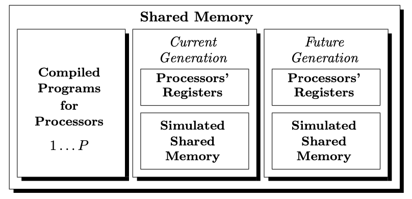
Shared memory structure for simulations

Fault-tolerant version

after this transformation can execute fault-free PRAM programs in presence of failures
the fault free program is the input to the interpreter

Transformation steps

shared memory management:
- compiled PRAM program is stored in shared memory
- remaining shared memory is used to simulate shared memory of PRAM, containing two generations of memory (current and future)
- private registers of simulated processors are stored in each generation of simulated shared memory
  - private registers \(r\) use \(l = O(|r| \cdot N)\) memory cells
- current memory is used for reads, future memory for writes
- all memory references are made using generation subscript 0 or 1
- asymptotic memory requirement is \(O(m+l)\)

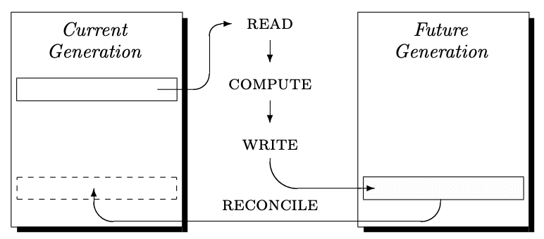
Memory that can be read by processors is not changed until it is safe to do so → results in idempotent PRAM instructions enabling (possibly) multiple executions.

Simulation proceeds for each parallel step until simulated PRAM halts as follows:

each simulated PRAM step is executed (by performing read/compute/write as necessary)
current and future memories are reconciled by copying changed cells and new register values from future to current (to produce new current memory)
simulated instruction counter has value 0 to indicate halting

Processing within simulation step

Pseudocode

for an interpreter using 2 generations of memory

forall processors PID= 1..P parbegin
    shared SM[0..1, 1..m];
    shared PROG[1..N, 1..size];
    shared IB[1..N ];
    shared r[0..1, 1..N ] of                // two sets 
        record IC, RB, WB, ... end          // of registers

    // Initialize instruction counters
    r[0,pid].IC := 1;                       // start at first instruction

    while r[0,pid].IC != 0 do               // while not HALT

        // Tentative computation
        IB[pid] := PROG[pid,r[0,pid].IC];   // fetch R,C,W,J
        r[1,pid]:= r[0,pid];                // copy registers
        r[1,pid].RB := SM[0,[R (r[1,pid])]  // read cycle
        r[1,pid] := C(r[1,pid]);            // compute cycle
        SM[1,W(r[1,pid])] := r[1,pid].WB    // write cycle
        r[1,pid].IC := J(r[1,pid]);         // next instruction

        // Reconcile shared memory
        SM[0,W(r[1,pid])] := SM[1,W(r[1,pid])]; 

        // Reconcile registers
        r[0,pid] := r[1,pid] 
    od
parend

Write-all algorithm is used to execute each 4 actions in the work phase → assures that actions of given phase are performed before actions of the next phase are attempted
Typical write-all uses \(\Theta(N)\) memory and \(P \leq N\) processors
- do not need to be \(P=N\) wince write-all will assign processors to tasks
Memory needs to be cleared when running write-all consecutively
- utilize two workspaces of size \(\Theta(N)\): H1 and H2
- use one workspace and clear the other; at the same time, during simulation
- has no asymptotic impact on memory usage or efficiency of robust algorithms
Lastly check for termination: processors examine simulated ICs and write halt = false is \(IC \neq 0\)

Pseudocode for fault-tolerant PRAM interpreter

forall processors PID=1..P parbegin
    shared PROG[...], SM[...], IB[...], r[...]

    // two auxiliary workspaces of size Theta(N)
    shared H1, H2;     

    // termination flag
    shared HALT initial false;   

    a: Initialize ICs to 1 and clear H2 using H1;

    // while not all processors halted
    while not HALT do           
        b: Perform a tentative pram step and clear H1 using H2; 
        c: Reconcile shared memory and clear H2 using H1;
        d: Reconcile registers and clear H1 using H2;
        e: Compute: HALT=false iff exists PID : IC[PID] != 0
             and clear H2 using H1; 
    od
parend.

Analysis

let \(S_{N,P}\) be work of solving write-all of size N using P \(P \leq N\) processors
complexity of applying single PRAM step in bounded by:
- complexity of solving write-all in steps a, c, and e
- complexity of robustly writing and copying \(l = O(|r| \cdot N) = O(N \log^{k}n)\) shared memory in steps b and d
to copy \(l\) memory, apply write-all \(l/N\) times at cost \(S_{N,P}\)
total cost of one PRAM step is:

\(S = O(S_{N,P} + (l/N)S_{N,P})\)

\(= O(S_{N,P} + |r|S_{N,P})\)

\(= O(S_{N,P} + \log^k{n} \cdot S_{N,P})\)

\(= O(S_{N,P} \cdot \log^k n)\)

Simulation Cost Theorem

Cost of simulating a single parallel step of \(N\) fault free processors, each using \(L\) private registers, on \(P\) fail-stop processors in failure model \(F\) is \(O(S_{N,P} \cdot L)\) where \(S_{N, P}\) is the work complexity of solving the write-all problem of size \(N\) in \(F\) using \(P\) processors.

When PRAM dies not need additional private memory cost of PRAM step simulation is \(O(S_{N,P})\).

General Simulations

Simulations for different failure models.

Initial failures

More simple simulation:

can bypass most steps used by fault-tolerant PRAM interpreter
use algorithm E to simulate on fail-stop PRAMs subject to initial failures

Algorithm E uses enumeration phase E1 to determine active processors. The remaining simulation contains a loop in which:

\(P\) processors use two generations of memory
to perform work of \(N\) simulated processors
each processor of \(P\) simulates \(N/P\) processors

Assume processors halt in synchrony, then:

Enumeration overhead (additive)
time overhead	\(O(\log N)\)
work overhead	\(O(P \log N)\)

Any \(N\)-processor, \(\tau\)-parallel-time EREW PRAM algorithm can be robustly simulated on a fail-stop EREW PRAM that is subject to static initial processor and initial memory faults. The work of the simulation is \(N \cdot \tau + O(P \log N)\), where \(P\) is the number of live processors.

Simulation subject to initial failures is optimal when \(N \cdot \tau = \Omega(P \log N)\).

Synchronous restarts

Use fault-tolerant PRAM interpreter to show robust and optimal simulations are possible → also applies when restarts allowed in synchrony at specific points e.g. next PRAM step.

Any \(N\)-processor EREW, CREW, or Common CRCW PRAM algorithm that uses arbitrary shared memory and polylogarithmic in the input size private memories can be robustly simulated on a fail-stop \(P\)-processor Common or Arbitrary CRCW PRAM when \(P \leq N\).

Any \(N\)-processor EREW, CREW, or Common CRCW PRAM algorithm can be optimally simulated (with constant overhead) on a fail-stop \(N\)-processor CRCW PRAM, when \(P \leq N \log \log N / \log^2 N\).

Detectable restarts

Any \(N\)-processor PRAM algorithm can be executed on a restartable fail-stop P-processor CRCW PRAM, with \(P \leq N\).

Each \(N\)-processor PRAM step \(i\) is executed in the presence of any pattern \(F_i\) of failures and detectable restarts of size \(M_i\) with:

Work, Overhead Ratio
work \(S\)	\(O(min\{N + P \log^2 N + M_i \log N, N \cdot P^{\log\frac{3}{2}}\})\)
overhead ratio	\(\sigma = O(log^2 N)\)

EREW, CREW, and Common CRCW PRAM algorithms are simulated on fail-stop Common CRCW PRAMS
Arbitrary CRCW PRAMS are simulated on fail-stop CRCW PRAMS of the same type

From this follows that:

when \(|F|\) is \(\Omega(N \log N)\) then \(\sigma\) is \(O(\log N)\)
when \(|F|\) is \(\Omega(N^{1.59})\) then \(\sigma\) is \(O(1)\)

Overhead ratio \(\sigma\) improves for large failure patterns.

Undetectable restarts + asynchrony

this model is essentially identical to PRAM model with asynchronous processor behavior and atomic memory read/write access → view disparity in processor speeds as failures.
in the presence of arbitrary asynchrony or when the restarts are undetectable, deterministic simulations become difficult due to the possibility of processors that are delayed by failures writing stale values to shared memory.
Simulation approaches using information dispersal techniques and randomization have been pursued for asynchronous settings.

Any \(N\)-processor, \(\log^{O(1)} N\)-time, \(m\)-memory PRAM algorithm can be (deterministically) simulated on a fail-stop \(P\)-processor CRCW PRAM (\(P \leq N\)) with undetectable restarts, and using shared memory \(m \cdot \log^{O(1)} N\). Each \(N\)-processor PRAM step is executed in the presence of any pattern \(F\) of failures and undetected restarts with \(S = O(N^\epsilon)\) for \(\epsilon > 0\).