23. Architectures
Mar 31, 2021
Hypercube Simulations
- \(L = \Theta(\lg P)\)
- \(T_{PRAM} = \Theta(\lg P)\)
- \(W_{PRAM} = \Theta(P \cdot \lg P)\)
- \(T_{Simulation} = \Theta(\lg^{2} P)\)
- \(W_{Simulation} = \Theta(P \cdot \lg^{2} P)\)
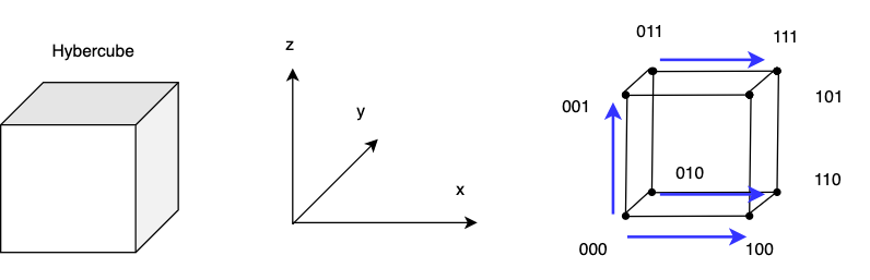
Associative operation on a hypercube
Consider an associative operation e.g. \(\sum x\) on a PRAM: oblivious simulation degrades by \(\log P\) factor.
There is better an oblivious simulation for this:
- send own value to specific dimension neighbor
- neighbor adds to own value
-
Step 1: send left to right, send in increasing order:
011→111: \(X_3 + X_7\)001→101: \(X_1 + X_5\)010→110: \(X_2 + X_6\)000→100: \(X_0 + X_4\)
-
Step 2 repeat operation, but now in y dimension
- those nodes that already contributed their value do not need to participate in the computation
100→110: \(X_0 + X_4 + X_2 + X_6\)101→111: \(X_1 + X_5 + X_3 + X_7\)
-
Step 3 only two nodes participate and add values in z-dimension
- result
110→111: \(X_0 + X_1 + X_2 + X_3 + X_4 + X_5 + X_6 + X_7\)
- result
The efficiency of this simulation is \(\lg P\), which is the same as the original algorithm → there is no loss in efficiency in this simulation.
Broadcast on a hypercube
Broadcast is another operation that is good on a hypercube
- within a hypercube, there exists an embedded tree structure
- there are many ways to use and interpret the architecture, here are two
- leaves are processors, the rest are switches
- all are processors
- hypercube allows simulating log-tree algorithms without overhead
- the weak point of this strategy is that root can become a bottleneck if all left nodes want to concurrently communicate with right side nodes → address such bottleneck by using a fat tree
Fat Tree
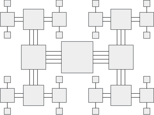
- make the fat tree strong node (center) the tree root
- less powerful nodes on sides with strong connecting wires
- nodes weaken over distance
- nodes can be understood as switches
- this architecture can be packed tightly on a plane and reduces the impact of bottleneck root, while preserving the tree structure
- it is easy to build and can be layered vertically also
Tree-connected grid / grid-connected trees
Consider 2D grid architecture:
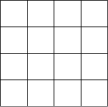
we are trying to look at each row and "plant a tree" over this row → plant a new tree over every row and column:
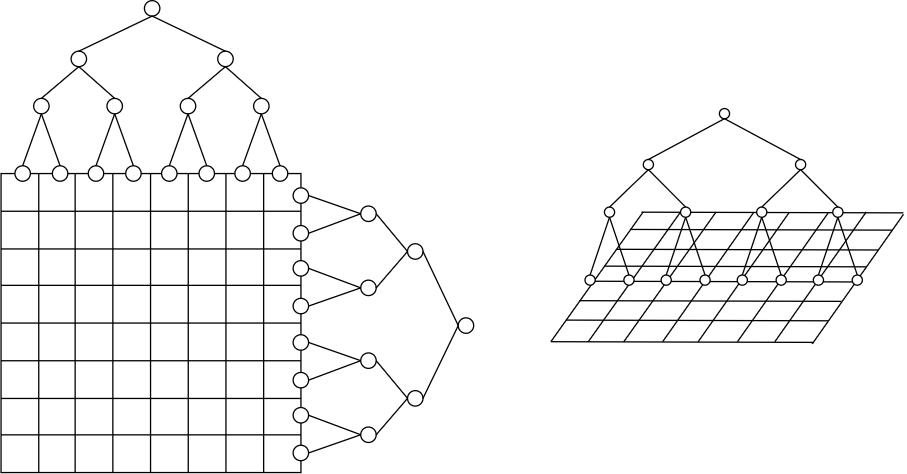
Message path is from node A to node B:
- if message path < \(\log\): send along tree
- if message path > \(\log\): send along the grid, do not overload the root.
- \(> \log\) implies we have to cross the root
- dot he same across every row and column
If there is not too much traffic, can reduce latency from \(P^2\) to \(\log P\)
- in worst case may not help
- amortized cost may be reasonable
Hardware cost: \(HW \$ = \Theta(P)\) + wires of the grid
Number of nodes: \(2 \cdot \sqrt(P) - 1 = \Theta(P)\)
Hardware cost of grid tree:
\(\Theta(P) + \#cols \cdot tree + \#rows \cdot tree = \Theta(P) + \sqrt{P} (\Theta(P)) + \sqrt{P} (\Theta(P)) = \Theta(P)\)
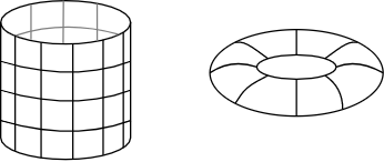
How to make sure grid behaves?
- roll into cylinder → longest path \(\sqrt{P} - 1\)
- shape like a bagel → max path cut into half \(\sqrt{P} / 2\)
- with the bagel shape all path distances are cut in half in \(x\) and \(y\) dimension
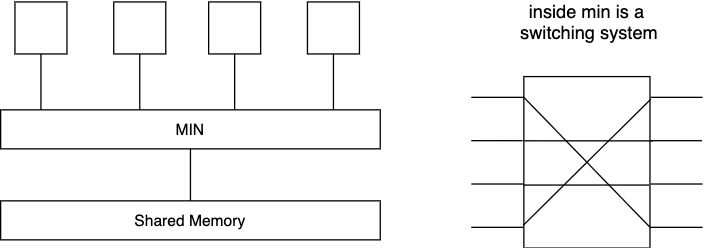
Multi-connection - Interconnection Network
- first introduced in telephony
- no contention → if wire is already in use set busy signal
- if not busy, allow routing any permutation A - B
- this signal has inspired icons for switches
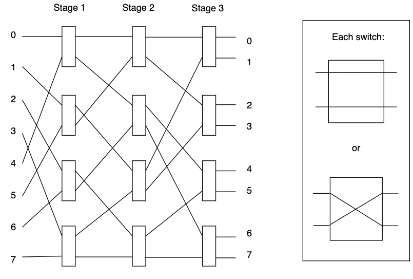
Omega/Shuffle Exchange
- Imagine the way of shuffling 8 cards → split into two then interleave them
- claim: will reach the destination → all paths 0...8 can reach 0...8 outputs
- within this tree is an embedded tree structure
- in \(\log\) time, can go from any input to any output
- 0: go north
- 1: go south
Can interpret the omega network/shuffle exchange as processors → memory
- the architecture works in both directions
- hardware cost \(HW \$ = \Theta(P) + \# \text{stages} \cdot \text{cost of stage} = \Theta(P) + \log_{2}P \cdot \frac{P}{2} = \Theta(P \lg P)\)
- if processors are expensive and switches are cheap, then this architecture may be worthwhile to use
- all paths have the same length → uniform min (uniform multi-connection network)
This architecture can perform summation task:
- sum all leaves → broadcast op-code to all leaves
- when memory gets the message, return memory value in opposite direction
- when switch receives a message, it sums the inputs
- requester receives the result in \(2 \cdot \log P\) time
It can do any associative operation this way at no delay relative to the PRAM because it is tailored to this architecture
Simulation using shuffle exchange:
- \(T_{PRAM} = \Theta(\lg P)\)
- \(W_{PRAM} = P \cdot \Theta(\lg P) = \Theta(P \lg P)\)
- \(T_{sim} = \Theta(\lg P)\)
- \(W_{sim} = HW \$ \cdot \Theta(\lg P) = \Theta(P \lg^2 P)\)