PRAM Algorithms

Programming for PRAM

usual representation is a high-level program that can be compiled into assembly level PRAM instructions
many techniques exist for compiling such programs → does not affect computational complexity of algorithms
programs are model independent
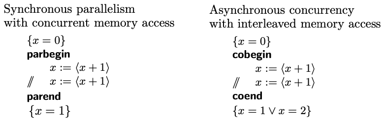
parbegin - parend indicate parallel blocks
concurrent executions in sync/async parallel models have differences
sync will perform concurrent execution
async will interleave actions in some order

In this example (CRCW PRAM) statements marked with // are executed concurrently

typically processors are running the same program
SPMD = single-program multiple-data = model where processors have their on instruction counters and maybe working on different data

Example of SPMD program where each processor executes the sequential Program(pid):

forall processors pid = 1..P parbegin
    Program(pid)
parend

alternative notion of the same:

parbegin
 Program (1) // Program (2) // ... // Program(P)
parend

SPMD model requires special attention when dealing with if-else or while-do statements, including precisely defining specific timing of operations for the program to make sense

In example below: - right-hand side is evaluated first, assignment last - pre and post conditions hold - assume identical timing for all instructions

{x = 1 && y = 2}
forall processors pid = 1..2 parbegin
    if pid = 1
    then x:= y * y + x
    else y := 0 fi
parend
{x = 5 && y = 0}

Spanning Tree Broadcast

assume spanning tree with depth \(d\) is known in advance
each processor has a channel to its parent and children
root \(p_i\) sends a message \(M\) to its children, who in turn send it to their children
this algorithm is correct for sync/async systems and message and time complexities are same

for \(p_i\)

upon receiving no message:
    terminate

for \(p_j, 0 \leq j \leq n-1, j \neq i\)

upon receiving M from parent:
    send M to all children
    terminate

Bounds
\(O(n-1)\)	message complexity
\(O(d)\)	time complexity

Parallel Tree Traversal

setup: sync parallel processors with shared memory operating on binary trees
store tree in an array to create maintenance-free tree:

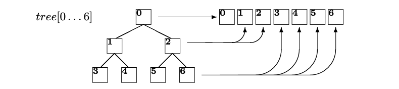
complete tree with \(n\) leaves is represented as a linear array \(tree[0\dots2n-2]\)
- root is at \(tree[0]\)
- any non-leaf at \(tree[i]\) has left child at \(tree[2i+1]\) and right child at \(tree[2i+2]\)
- use padding if number of children is not a power of 2
This representation can be generalized to \(q\)-ary trees: non-leaf has \(q\) children whose indices are \(qi+1, qi+2, \dots ,qi+q\)
use bottom-up or top-down traversal of tree
- number of leaves is proportional to size of input \(N\)
- height of tree is \(\log N\) (assume constant degree)
- traversal takes logarithmic time

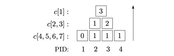
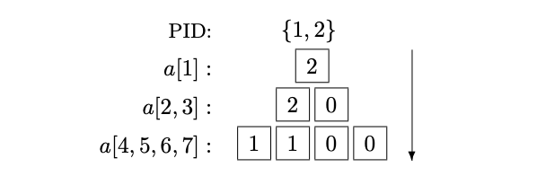
Parallel counting example

example of progress tree often used with divide-and-conquer
each processor writes into the node in the tree the sum of the two child locations
root node has final value 3
PID 1 is not necessary

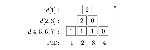
Progress evaluation example

Each processor writes 1 into leaf if it finished its task
sum of children stored in the parent
when value at root node is \(< N\) not all tasks completed

Load balancing example

two processors start from top
both proceed to right subtree because left subtree is complete, none on right is complete
in next step the processors divide equally to \(a[6]\) and \(a[7]\)

Processor Enumeration Algorithms

goal: enumerate participating processors
each uses an auxiliary tree data structure
each processor can call the algorithm procedure from a high-level program (same for all)
progress is measured in progress tree \(d\) where each subtree contains the number of completed tasks in its subtree, resulting in a summation tree

Using clear memory

assume clear shared memory, i.e. all tree nodes are initialized to 0's
perform bottom-up traversal to compute number of active processors
each active processor writes 1 in leaf \(c[PID + N - 2]\)
inactive processors do nothing
enumerate active processors to the left

procedure Enumerate1(integer pid, integer pn)
        shared integer
            c[0..2N - 2] init 0,
        private integer
        j1, j2,
        t;
    begin
        j1 := pid + (N - 2);
        pn := 1;
        c[j1] := 1;
        for 1...log(N) do
            t := (j1 - 1) div 2;
            if 2 * t + 1 = j1
                then j2 := j1 + 1
                else j2 := j1 - 1
            fi
            c[t] := c[j1] + c[j2]
            if j1 > j2
                then pn := pn + c[j2]
            fi
            j1 := t
        end for
    end.

Using timestamps

same as previous with the additional use of timestamps to ensure fresh values
allows reuse of the same tree over time
counts that are out of date are treated as 0s

procedure Enumerate2(integer pid, integer step, integer pn)
        shared integer
            c[0..2N - 2],
            cs[0..2N - 2];
            step init 0
        private integer
            j1, j2,
            t;
    begin
        step := step + 1;
        j1 := pid + (N - 2);
        pn := 1;
        c[j1] := 1;
        cs[j1] := step;
        for 1...log(N) do
            t := (j1 - 1) div 2;
            if 2 * t + 1 = j1
                then j2 := j1 + 1
                else j2 := j1 - 1
            fi
            if cs[j1] = cs[j2]
                then c[t] := c[j1] + c[j2]
                    if j1 > j2
                        then pn := pn + c[j2]
                    fi
                else c[t] := c[j1]
            fi
            cs[t] := step;
            j1 := t
        end for
    end.

Clearing old data

clear memory before using it
assume there are no active siblings at any tree node by clearing the subling and writing the new value in current location in c

procedure Enumerate3( integer pid, integer step, integer pn)
        shared integer
            c[1..2N - 2]
        private integer
            st,
            j1,j2,
            t;
    begin
        j1 := P ID + (N - 2);
        pn := 1;
        st := 1;
        for 1...log(N) do
            t := (j1 - 1) div 2;
            if 2 * t + 1 = j1
                then j2 := j1 + 1
                else j2 := j1 - 1
            fi
            c[j2] := 0;
            c[j1] := st;
            if j1 > j2
                then pn := pn + c[j2]
            fi
            st := c[j1] + c[j2];
            j1 := t
        end for
    end.

Load Balancing

uses a progress tree
number processors starting with 1 and refer to this number (instead of pid)
processors traverse the tree from root to leaf and allocate themselves to left/right subtree relative to incomplete tasks
at leaf processor computes index \(k\) of task to perform

procedure Progress(integer k, boolean done)
    shared integer array
        d[1..2N - 1];
    private integer
        i1, i2
        t;
    begin
        i1 := k + (N - 1);
        if done
           then d[i1] := 1;
        else d[i1] := 0;
        fi
        for 1...log(N) do
            t := (i1 - 1) div 2
            if 2 * t + 1 = i1
                then i2:=i1 + 1
                else i2:=i1 - 1
            fi
        end do
    end.

Broadcast with Tree

for CREW PRAM for broadcasting value to all processors
for simplicity assume \(P = 2^k-1\) for some \(k > 0\)
processor PID = 1 will broadcast the value
for any node in the tree, \(B[j]\), its parent is \(B[j / 2]\)
start by having processor 1 write its value to root, then children read the value from their parent progressively
note concurrent reads → can be modified to have parent push a value to its children to achieve EREW model which does not impact complexity

Bounds
\(\Theta(\log p)\)	time complexity
\(\Theta(P \log P)\)	work

procedure Divide-and-Conquer(integer pn, integer P, integer k)
    shared integer array
        c[0..2N - 2],
        d[0..2N - 2];
    private integer
        j, j1, j2;
        j := 0;
        size := N;
        c[0] := P;
    begin
        while size != 1 do
            j1 := 2 * j + 1; j2 := 2 * j + 2;
            c[j1] := c[j] * (size/2 - d[j1]) div (size - d[j]);
            c[j2] := c[j] - c[j1];
            if pn <= c[j1]
                then j := j1
                else j := j2; pn := pn - c[j1]
            fi
            size := size div 2
        end do;
        k:=j - (N - 1)
    end.

Modified version of Divide-and-Conquer method to perform broadcast with tree, where parent pushes value to its children

forall processors pid = 1..P parbegin
    shared B[1..P ]
    if pid = 1 then B[1] := value fi
    for h = 0 to floor(log P) - 1 do
        if 2^h <= pid < 2^(h+1) then
            B[2pid] := B[pid]
            B[2pid + 1] := B[pid]
    end do
parend.

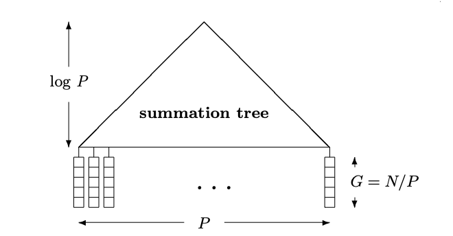
Optimal Parallel Summation

this example is for summation but can be applied to any associative operation
goal: combine optimal sequential algorithm for summation with fast parallel algorithm for summation
let
- \(N\) — size of input
- \(P \leq N\) — number of processors, instance size, number of leaves
- \(\log P\) — height of tree
- \(G = N/P\) — size of input mapped to each leaf ("chunk")
each processor at leaf will compute \(G\) input elements using sequential algorithm.
for optimal work, choose parameters such that \(W = \Theta(N)\)

Data structure for summation

Bounds
\(\Theta(\log N)\)	time complexity
\(\Theta(N \log N)\)	work
\(\Theta(P / \log P)\)	speedup