9. Failure Models
Feb 10, 2021
Failure Models
Recall PRAM model: synchronized, high bandwidth, no failures. Now remove assumption of no failures and assume there is some adversary working against us.
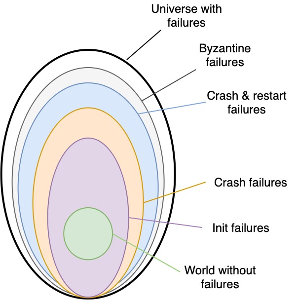
| Failure type | Description |
|---|---|
| init | processor fails to start |
| crash | processor stops, doesn't do anything else after that |
| crash & restart | processor crashes but can restart |
| byzantine | adversary can cause any arbitrary behavior |
There are more failure models: omission failure, transient failure, software failure, security failure, temporal failure, environmental perturbations, but omission failure occurred while taking notes.
Failure model - what type of crashes occur during computation - is adversary online/offline: - online adversary can cause dynamic failures during computation - offline adversary must choose failure model before computation starts - number of failures \(f < P\) → some processor always survives - adversary is omniscient
Example: Enumeration with dynamic failures
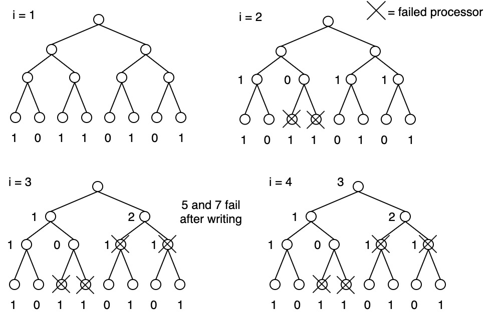
- processors zero memory before use, initially 3 failures occur
- 2nd pass: processors 2, 3 die
- 3rd pass: processors 5,7 die after clearing & writing
- final result overestimates number of available processors (real number: 1)
If there are dynamic failures during this computation, the result will be an overestimate
Overestimate is not bad; underestimate is bad. Why?
Consider \(N=1000\) and number of tasks 100. In both cases processor estimate is \(P = 10\):
- \(P\) is overestimate (actual \(P=2\)): \(W = 100 \times 2 = 200\)
(less work done than expected)
- \(P\) is underestimate (actual \(P=100\)): \(W = 100 \times 100 = 10,000\)
(more work done than expected)
With overestimate you can reallocate remaining work if all tasks are not done, but will not end up doing unnecessary work. Enumerate processors and reallocate work.
Work with Failures
- in a non-failure environment, work \(W\) is the area of \(P \cdot T_P\)
- with failures time to completion increases with failures
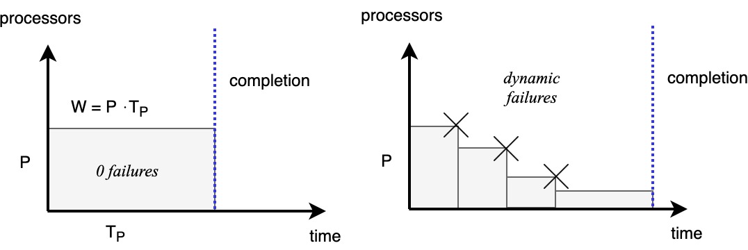
- with failures \(P \cdot T_P\) no longer a good way to estimate \(W\)
- commute the area under the curve into a step function to determine work: \(W = \sum_{1}^{T}(P_T)\) where \(P_t\) is the number of active processors at time \(t\).
Load Balancing Progress Tree
Given \(N\) tasks and \(P\) processors and \(N = P\), processors write 1 to the leaf when they are done with their task
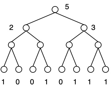
- Perform bottom-up simple addition:
- everywhere where 1: there is a processor
- everywhere where 0: processor failure
- Result: 5 tasks completed and 3 tasks remain
- Load balance the remaining tasks
Next: assume more processors fails after the first pass (tasks are done but processors are dead)
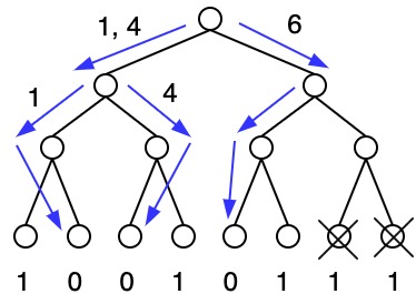
- Assume we now have 3 live processors \(P=3\) e.g. \({1, 4, 6}\)
- Look for the remaining tasks: \(8 - 5 = 3\) then use the same tree as a load balancing tree to find these 3 undone tasks
- iterate top to bottom:
- \(4 - 2 = 2\) tasks remain on left → send \(2/3\) of \(P\) this way
- \(4 - 3 = 1\) task remains on right → send \(1/3\) of \(P\) this way
- Repeat until finding the tasks