4. Analysing
Jan 25, 2021
Analysing parallel algorithms
Alarm Example
Consider the following algorithm:
1 2 3 4 | |
It may cause multiple alarms to sound at once.
Then compare to this version:
1 2 3 4 5 | |
Will only alarm once, but the algorithm is linear — not good.
Logical-OR on PRAM
Given array \(X[1...N]\), set \(r = 1\) if some \(X[i] = 1\) and 0 otherwise.
Sequential version
1 2 3 4 5 | |
Analysis of sequential version time: - lower bound \(\Omega(N)\) - upper bound \(O(N)\) - → sequential time complexity is \(\Theta(N)\) - this is time-optimal implementation \(T_1^*\)
Parallel version
\(r\) is in shared memory, initialized to 0, \(N = P\)
1 2 3 4 5 6 | |
Parallel version analysis: - \(T_P(N) = \Theta(1)\) - \(S = \frac{T_1^*}{T_P(N)} = \frac{\Theta(N)}{\Theta(1)} = \Theta(N) = \Theta(P)\)
- \(T\) describes time and number of machine instructions (effort)
- Work = \(W = P \cdot T_P\) - processors \(\times\) time product
- \(T_1(N)\) - time on a single processor
- superlinear speedup may occur due to caches but not realistic otherwise, because it would imply there is some \(T_1 > T_1^{*}\) and we should always use \(T_1^{*}\)
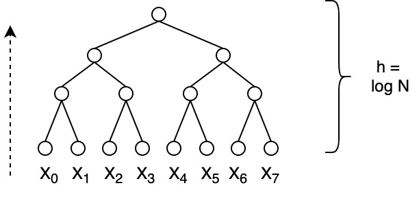
Parallel Sum
This example is for summation but can be done with any associative operation e.g. \(\times\), and, or, max, min...
Setup have \(X[1...N]\) → want \(\sum_{1}^{N} X[i]\)
- Create a summation tree
- this is a binary tree with \(N\) leaves and \(h = \lg N\)
- initialize leaves with values of \(X\)
- sum children bottom to top; store value at parent
In code map the tree to an array then sum with neighbor:
| Bounds |
|---|
| \(T_P(N) = \Theta(\lg N)\) |
| \(S = \frac{T_1^*(N)}{T_P(N)} = \frac{\Theta(N)}{\Theta(\lg N)} = \Theta(\frac{N}{\lg N}) < \Theta(P)\) |
| \(W = P \cdot T_P = N \cdot \Theta(\log N) = \Theta(N \lg N) > \Theta(N)\) |
- algorithm is log-efficient when \(P \cdot T_P = O(T_1^*(N) \cdot \lg N)\)
- work is polylog efficient when \(P \cdot T_P = O(T^*_1 \cdot \lg^k(N))\) where \(k\) is some constant
- work is optimal when \(P \cdot T_P = O(T_1^*(N))\)
optimal work implies linear speedup
Example when \(N=1024\)
- \(T_1^*(N) = 1024\)
- \(T_P(N) = \lg N = 10\)
- \(S = 1024/10 > 100\)x speedup