Agglomerative
Summarized notes from Introduction to Data Mining (Int'l ed), Chapter 5, section 3
Unsupervised learning > clustering
-
two basic strategies to producing hierarchical clusters:
- agglomerative: start with points as individual clusters then merge closest pair of clusters (more common)
- divisive: start with on all-inclusive cluster, then split until only singleton clusters remain
-
point distances are computed and represented in a distance matrix
-
dendrogram is used for visualizing hierarchical clusters (see: example)
-
captures cluster relationships and their merging/split order
-
for 2D points, it is also possible to visualize using nested cluster diagram
-
Pseudo code
1 2 3 4 5 6 | |
Proximity metrics
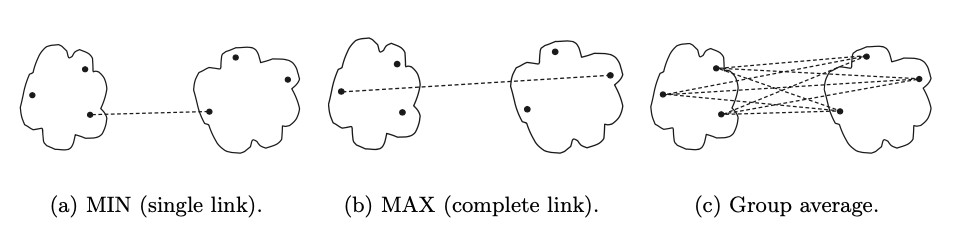
| Metric | Description |
|---|---|
| Min / single link | distance between two closest points |
| Max / complete link / (clique) | distance between two farthest points |
| Group average | average pair-wise proximity between points |
| Centroid | distance between two centroids |
| Ward's method | increase in SSE after merging two clusters |
- Single link is good for handling non-elliptical shapes, but sensitive to noise and outliers
- Complete link is less susceptible to noise and outliers, favors globular shapes, and can break large clusters
-
Group average, where \(m_k\) is number of objects in cluster \(C_k\):
\(\displaystyle \text{proximity}(C_i, C_j) = \frac{\sum_{x \in C_i, y \in C_j} proximity(x, y)}{m_i \times m_j}\)
-
Ward's method (same objective as K-means) => mathematically very close to group average when the distance in group average is taken to be the squared distance of points
General case: these proximity metrics represent different choices of coefficients to Lance-Williams formula.
Example
Consider distance matrix of points:
1 2 3 4 5 6 7 | |
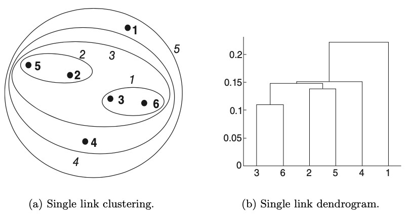
Single-link/MIN distance
\(d(\{3,6\}, \{2,5\})\) = \(min \big(d(3,2), d(6,2), d(3, 5), d(6, 5) \big)\)
\(= min(0.15, 0.25, 0.28, 0.39)\) = \(0.15\)
Complete-link/MAX distance
\(d(\{3,6\}, 4)\) = \(max \big(d(3,4), d(6,4)\big)\) = \(max(0.15, 0.22)\) = \(0.22\)
\(d(\{3,6\}, \{2,5\})\) = \(max(0.15, 0.25, 0.28, 0.39)\) = \(0.39\)
=> cluster \(\{3,6\}\) will be merged with 4, because its max distance is lower.
Group average
\(d(\{3,6, 4\}, 1)\) = \((0.22 + 0.37 + 0.23)/(3 \times 1)\) = \(0.28\)
\(d(\{2,5\}, 1) = (0.24 + 0.34)/(2 \times 1)\) = \(0.29\)
\(d(\{3,6, 4\}, \{2,5\})\) = \((0.15+0.28+0.25\) \(+0.39+0.20+0.29)/(3 \times 2)\) = \(0.26\)
=> clusters \(\{3,6, 4\}\) and \(\{2,5\}\) are merged since their group average is lowest.
Nested-clustering diagram and dendrogram
Cluster sizes
For proximity metrics that involve sums (e.g. group average, Wards, centroids) there are two approaches:
- weighted: all clusters treated equally (points in different clusters have different weight)
- unweighted: considers number of points in each cluster (all points have same weight)
In general unweighted approach is preferred unless there is some reason to weight individual points differently (e.g. due to uneven sampling).
Analysis
Complexity
\(m\) - data points
| Time (optimal) | \(O(m^2 \lg(m))\) |
| Time, general | \(O(m^3)\) |
| Space (proximity matrix) | \(O(m^2)\) |
Advantages
-
avoid difficulties of choosing initial points, number of clusters
-
able to discover hierarchical relationships
-
clusters correspond to meaningful taxonomies
Limitations
-
lack of global objective function
- there is no global objective being optimized
- clustering decisions are made locally at each iteration step
-
merging/splitting decision are final
- local optimization cannot be applied globally
- rearranging branches, or using K-means to form initial small clusters before hierarchical clustering, can reduce impact of this limitation
-
computationally expensive: time and space complexity limits the size of data sets that can be processed
-
outliers impact depends on choice of proximity metric:
- difficult for Ward's method and centroid-based hierarchical clustering because they increase SSE and distort centroids
- less problematic for min, max, and group average
- outliers can be removed to avoid these issues