21. Zero-time sorter
Mar 24, 2021
ABD performance
There are two considerations
- safety == correctness
- liveness (related to performance)
Another related notion: wait-freedom: every operation always terminates, regardless of the relative speed of the processes.
The ABD algorithm says it is wait-free (it is not) → wait freedom cannot depend on failure. ABD is actually discussing conditional performance:
Required: \(f < \frac{N}{2}\) or 1 quorum survives
Read and write have two phases:
- query/get phase: broadcast, responses
- propagate/put phase: broadcast, responses
Each operation terminates because a majority is guaranteed to respond eventually.
ABD algorithm makes no assumptions about timing and when things will happen
Looking at conditional performance:
- an external observer can observe the system
- we can assume upper bound on message delays d, which is not known to the algorithm
- worst case broadcast delay is \(d\)
- max response delay is \(d\)
- 1 round of communication is \(2d\) total
- reads and writes are \(4d\) total (MWMR)
We also assume local processing time is 0 because network delays are significantly higher. But this is not always the case (cf. Dutta & co). Reads/writes sometimes take longer because local computation is computationally exhaustive. Read/write delay is actually \(2d\) \(+\) local computation (LC). As long as \(d > LC\) message latency is dominant and we can ignore \(LC\).
Zero Time Sorter
Recall linear/systolic array

- \(HW\$ = \Theta(P)\)
- Latency \(L = O(P)\) for reads and writes
Due to this latency, this architecture is not good for general purpose use, but it is good for special cases.
Phase 1: inputs arrive left-to-right
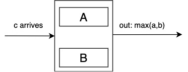
When \(c\) arrives, \(max(a,b)\) moves right anc \(c\) takes its place. If \(a\) or \(b\) is empty, \(c\) moves into empty place and nothing moves out. If both spots are empty, put \(c\) in either one of the empty spots.
Phase switch occurs whern there are no more empty slots and the array is full.
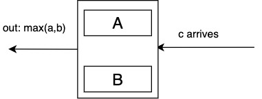
Phase 2: inputs arrive right-to-left
When \(c\) is arrived, send to left the minimum of \((a, b)\).
Memory capacity is \(2P\), e.g. \(P=4\) can sort 8 inputs.
This sort is called "zero time" because as soon as the last input is read in, the minimum pops out. In reality the sort takes \(2N\) steps.
Example
input: 67518423
1 2 3 4 5 6 7 8 9 10 11 12 13 14 15 16 | |
Analysis
- input size \(N = 2P\)
- \(T_P = N + N = \Theta(N)\)
- \(W = P \cdot T_P = \Theta(N \cdot P) = \Theta(N^2)\)
- \(T_1^* = \Theta(N \log N)\)
What is the relation \(W_P\) \(?\) \(T_1^*\)
\(O(N \log N \cdot \frac{N}{\log N}) = \Theta(N^2)\)
Overhead is \(\frac{N}{\log N}\)
Speedup: \(\displaystyle S = \frac{T_1^*}{T_P} = \frac{\Theta(N \log N)}{\Theta(N)} = \Theta(\log N)\)
Is this alog optimal, locarithmic or polynomially efficient? No. theoretically this is not interesting; but in practice it is: cheap and easy to build and logarithmic speedup.
2T Array
Recall crossbar architecture:
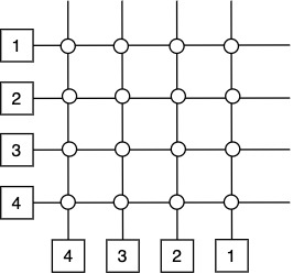
Number of switches is \(\Theta(N^2)\). Next idea: make switches into processors since they are expensive. This is called a 2T array.
Benefits: preserves simplicity and allows source routing
Source routing in 2T array works my looking at source \((a, b)\) and destination \((c, d)\).
For example go from (4,1) to (3,2): if column is less, move left, if row is less, move up. It is also allowed to move by row first then column, to balance the load in the wires. Minimum distance is the same either way.
Ideal considerations: building bigger systems out of smaller components.
- in a systolic array: number of wires = 2 (call this vertex degree)
- for 2T array vertex degree is 4
2T array hardware cost: \(HW\$ = \Theta(P) + \Theta(4 * P) = \Theta(P)\)
- The shape is a \(\sqrt{P} \times \sqrt{P}\) matrix
- Latency \(L = (\sqrt{P} - 1) + (\sqrt{P} - 1) = 2 \cdot (\sqrt{P} - 2) = \Theta(\sqrt{P})\)
Improvement from linear latency to \(\sqrt{P}\) latency
Simulation efficency
Const of simulating one PRAM step: all processors do R/W
- \(T_P = \sqrt{P}\)
- \(T_{sim} = T_P \cdot \Theta(\sqrt{P})\)
- \(W_{sim} = (P \cdot T_{sim}) = \Theta(P \sqrt(P) \cdot T_P)\)
Is this good simulation work efficiency? No but there may be some use cases.
PRAM is
- optimal when \(P \cdot T_P = O(T_1^*)\)
- log efficient when \(P \cdot T_P = O(T_1^* \cdot \log N)\)
- \(\Theta(P \sqrt(P) \cdot T_P) = W_P \cdot \sqrt{P}\) → polynomial overhead (overhead is \(P^\epsilon\))
This may be good (or not) based on practical considerations.
When \(P \leq N\) and \(P \cdot T_P = \Theta(T_1^* \cdot P^\epsilon)\)
\(P^\delta = P^{\epsilon + \frac{1}{2}}\)
- if \(\epsilon < \frac{1}{2}\) → polynomially efficient
- if \(\epsilon > \frac{1}{2}\) → not efficient at all