Basics

Summarized notes from Introduction to Data Mining (Int'l ed), Chapter 5

• Basic clustering problem

  • given: set of objects $X$, inter-object distances $D(x,y)=D(y,x)x,y\in X$
  • output: partition $P_D(x)=P_D(y)$ if $x,y$ are in the same cluster

• divide data into meaningful and/or useful groups, to describe or summarize data

  • clusters describe data instances with similar characteristics
  • ideally: small distance between points in cluster; long distance between clusters

• Some utility applications: data summarization, compression, efficiency in finding nearest neighbors

• clustering problem is very much driven by specific choice of algorithm

Clustering techniques

• based on nesting of clusters:

  • partitional (un-nested): divides data into non-overlapping clusters such that each instance is in exactly one cluster
  • hierarchical (nested): clusters are permitted to have sub-clusters; can be visualized as a tree

• based on count of instance memberships:

  • exclusive: each instance belongs to a single cluster
  • overlapping / non-exclusive: instance can belong to more than one cluster
  • fuzzy / soft: (probabilistic) instances membership in each cluster is determined by weigh 0-1, and typical additional constrain requires sum of weights equal to 1 => convert fuzzy to exclusive by assigning each object to cluster with highest weight

• based on instance membership in any cluster:

  • complete: each instance is assigned to some cluster
  • partial: not all instances are assigned a cluster; primary motivations include omitting noise and outliers

Types of clusters

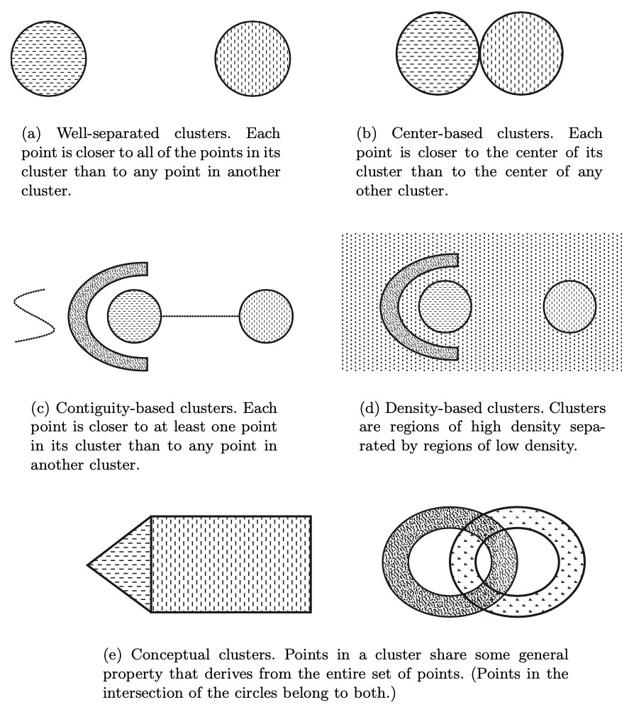
• well-separated: the distance between clusters is larger than distance between any two points within a cluster

• prototype-based / center-based: prototype defines a cluster and each object in cluster is closer to prototype that defines the cluster than to prototype of any other cluster; the prototype may be actual record or the calculated centroid

• contiguity-based / nearest neighbor / transitive: each point in a cluster is closer (or more similar) to one or more other points in the cluster than to any point not in the cluster.

• graph-based: nodes represent data objects, and edges their connections; cluster is a connected component where each node is connected within cluster but there are no connections to outside the cluster => when nodes are strongly connected, then the nodes form a clique

• density-based: cluster is dense region surrounded by a region of low density => useful strategy when clusters are irregular, intertwined or when noise or outliers are present

• shared-property/conceptual clusters: objects in a cluster share some common property; this encompasses all of the above, but enables defining clusters not covered by previous definitions.

Clustering properties

• Richness: for any assignment of objects to clusters there is some distance matrix $D$ such that $P_D$ returns that clustering $\mathrm{\forall }C\mathrm{\exists }D{P}_D=C$

• Scale-invariance: scaling distances by a positive value does not change the clustering $\mathrm{\forall }D{\mathrm{\forall }}_{K>0}{P}_D=P_{KD}$

• Consistency: shrinking intra-cluster distances and expanding inter-cluster distance does not change the clustering $P_D=P_{D^{\prime }}$

Impossibility theorem: no clustering algorithm can have all 3 properties.

Other considerations:

• order dependence: whether results differ based on the order of processing of data points
• nondeterminism: whether different runs give different results
• scalability: how large datasets the clustering algorithm can reasonably handle
• parameter selection: number of parameters and selection of optimal parameter values

Algorithms

Algorithm	Description	Category	Time Complexity (optimal)	Space Complexity
K-means	Find $K$ clusters represented by centroids	prototype-based, partitional, complete	$O(IKmn)$	$O((m+K)n)$
Agglomerative hierarchical clustering	Find hierarchical clusters by merging clusters	prototype-based / graph-based, hierarchical, complete	$O(m^2\lg (m))$	$O(m^2)$
DBSCAN	Cluster by density, ignoring low-density regions	Density-based, partitional, partial	$O(m\log m)$	$O(m)$
Fuzzy C-means	Points have weighted membership in clusters	prototype-based, partitional, fuzzy	$O(LKI)$	$O(LK)$

where: $m$ = number of points (records); $n$ = number of attributes; $I$ = number of iterations until convergence; $K$ = number of clusters, $L$ is the number of links

Also see:

• Expectation Maximization - statistical approach using mixture models
• Single-linkage clustering (SLC) - special case of agglomerative using single-link
• Self-organizing maps - clustering and data visualization based on neural networks

Cluster Validation

Some considerations:

• clustering tendency - distinguishing if non-random structure actually exists in the data
• determining correct number of clusters
• Evaluating how well the results of a cluster analysis fit the data without reference to external information.
• Comparing the results of a cluster analysis to externally known results, such as externally provided class labels.
• Comparing two sets of clusters to determine which is better

Defining cluster evaluation metrics is difficult, there are 3 general categories:

1. unsupervised: measure goodness without reference to external information (e.g. SSE); two subclasses:

   • cohesion: compactness, tightness - how closely related objects in a cluster are
   • separation: isolation - how distinct or well-separated clusters are

2. supervised: measures the extent to which the clustering structure discovered by a clustering algorithm matches some external structure (e.g. entropy of class labels compared to known class labels)

3. relative: Compares different clusterings or clusters, using either supervised or unsupervised metrics

Unsupervised

Cohesion and separation

• for graph-based view of cohesion/separation:

  • ${\displaystyle \text{cohesion}(C_i)}$ = $\sum _{x\in C_i,y\in C_i}proximity(x,y)$
  • ${\displaystyle \text{separation}(C_i,C_j)}$ = $\sum _{x\in C_i,y\in C_j}proximity(x,y)$

• proximity function can be similarity or dissimilarity

• If clusters have prototype (centroid or menoid)

  • cohesion and separation can be defined as distance from prototype:
    ${\displaystyle \text{cluster SSE}}$ = $\sum _i\sum _{x\in C_i}distance(c_i,x{)}^2$

  • Group sum of squares (SSB) measures distance between clusters
    ${\displaystyle \text{Total SSB}}$ = $\sum _{i=1}^K{m}_i\times distance(c_i,c{)}^2$

The result of cohesion/separation can be used to improve clustering by merging or splitting clusters

Silhouette Coefficient

• Evaluation metric for evaluating points in a cluster. Steps:

  • Calculate $a_i$, which is the average distance from object $i$ to all other objects in its cluster

  • Calculate $b_i$, which is the minimum average distance from object $i$ and objects in any cluster not containing $i$

  • The silhouette coefficient is: $s_i=(b_i-a_i)/max(a_i,b_i)$

• The range of coefficient is -1 to 1. Negative value is bad; as high as possible is good (obtained when $a_i=0$).

• Cluster S.C. can be computed by taking the average S.C. of its points
• Does not work well on arbitrary shapes.

Cophenetic Correlation Coefficient (CPCC)

Cophenetic Correlation Coefficient (CPCC) metric is for evaluating hierarchical clustering

• cophenetic distance between two objects is the proximity at which an agglomerative hierarchical clustering technique puts the objects in the same cluster for the first time
• CPCC calculates the difference between cophenetic distance and original distance matrix

Supervised

• supervised methods include knowing the real cluster data labels
• can help establish "ground truth" for clustering results
• similar metrics can be defined for precision, recall and F-measure

Entropy

• measure the degree of clusters matching known class labels

• For a set of clusters, $e$:

  ${\displaystyle e=\sum _{i=1}^K\frac{m_i}{m}{e}_i}$

• For individual cluster, $e_i$:

  ${\displaystyle e_i=-\sum _{j=1}^L{p}_{ij}\lg p_{ij}}$

  where:

  • $L$ is number of classes
  • $p_{ij}=m_{ij}/m_i$
  • $m_i$ is number of objects in cluster $i$
  • $m_{ij}$ is number of objects of class $j$ in cluster $i$

Purity

• the maximum $p_{ij}$ for a cluster

• overall purity of a cluster is

  ${\displaystyle \sum _{i=1}^K\frac{m_i}{m}ma{x}_j(p_{ij})}$